FFT-Based Image Convolution: Theory, Algorithm, and Tradeoffs

This page explains FFT-based convolution as a reference technique.

It covers:

• why it works,
• how the algorithm is structured,
• why it changes performance characteristics,
• and what tradeoffs it introduces.

1. The Core Insight: Representation Matters

Naive convolution operates in the spatial domain:

• pixels interact with nearby pixels,
• work is repeated locally over and over again.

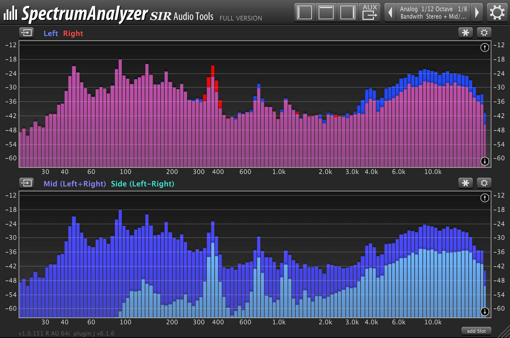
FFT-based convolution operates in the frequency domain:

• the image is represented as a combination of frequency components,
• global structure replaces repeated local work.

This change of representation is the key to improved performance.

2. The Convolution Theorem

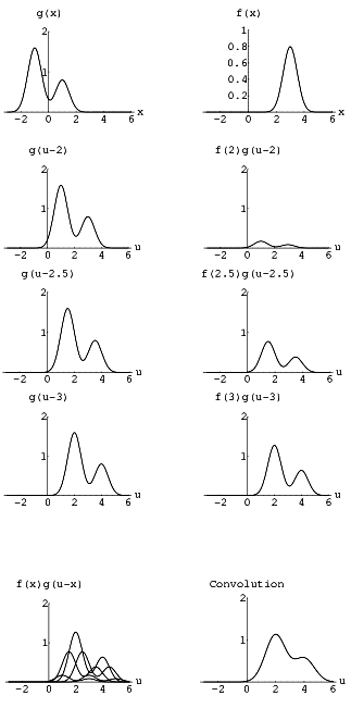
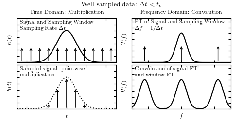
The convolution theorem states:

Convolution in the spatial domain corresponds to multiplication in the frequency domain.

Formally:

FFT(I * K) = FFT(I) · FFT(K)

This is a mathematical identity, not a programming trick.

It allows us to replace many local multiplications with:

• a small number of global transforms,
• followed by simple element-wise multiplication.

3. What the FFT Does (Conceptually)

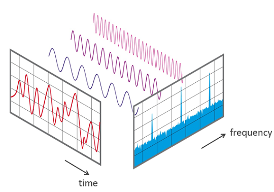
The Fast Fourier Transform converts a signal from one representation to another.

For images:

• spatial patterns become frequency components,
• local neighborhoods become global structure.

You do not need the mathematical derivation to understand the algorithmic effect:

Convolution becomes multiplication.

This is the transformation that makes FFT-based convolution attractive.

4. The FFT-Based Convolution Algorithm

A complete FFT-based convolution consists of these steps:

1. Padding
   The image and kernel are padded so that wraparound artifacts do not occur.
2. Forward FFTs
   A 2D FFT is applied to both the image and the kernel.
3. Pointwise Multiplication
   Corresponding frequency components are multiplied.
4. Inverse FFT
   The result is transformed back to the spatial domain.
5. Cropping
   The valid region is extracted to match the original image size.

Padding is essential.
Without it, the FFT computes circular convolution, which does not match the naive definition.

5. Computational Cost

FFT-based convolution runs in:

O(W · H · log(W · H))

Notice what is missing:

• there is no k² term.

Once the data is transformed, kernel size no longer dominates runtime.

This explains an important measured behavior:

• FFT is slower for small kernels (overhead dominates),
• FFT is much faster for large kernels.

6. Tradeoffs and Overhead

FFT-based convolution introduces costs that naive convolution does not:

• additional memory usage,
• complex arithmetic,
• non-local memory access patterns,
• setup and padding overhead.

These costs are real and measurable, which is why profiling is essential.

7. What Profiling FFT-Based Convolution Shows

Profiling FFT-based convolution typically reveals:

• FFT routines dominating runtime,
• clear algorithmic phases,
• relatively little time spent in kernel application itself.

This reinforces a central lesson:

Performance is shaped by algorithm structure, not by individual lines of code.

8. Why This Technique Matters Beyond Images

FFT-based convolution is important not because of image processing, but because it demonstrates a general principle:

Changing the representation of a problem can change its complexity.

Once you understand this example, you will recognize the same pattern in signal processing, numerical methods, physics simulations, and data analysis.