
Objective: By the end of this activity, you should will:
- Understand the structure and properties of a Binary Search Tree (BST).
- Learn how to add (insert) and delete nodes in a BST.
- Visualize tree transformations using graphs.
Activity Plan
1. Introduction to Binary Search Tree (10 minutes)
- BST Definition:
- A binary tree where each node has:
- A value greater than all values in its left subtree.
- A value less than all values in its right subtree.
- A binary tree where each node has:
- BST Properties:
- Efficient for search operations (O(log n) on average).
2. Insertion in BST (30 minutes)
- Insertion Algorithm:
- Start at the root.
- If the tree is empty, create a new node as the root.
- Compare the value to insert with the current node:
- Go left if smaller, go right if larger.
- Repeat until you find an empty spot, then insert the new node.
- Code Example (C++):
\struct Node {
    int value;
    Node* left;
    Node* right;

    Node(int val) : value(val), left(nullptr), right(nullptr) {}
};

Node* insert(Node* root, int value) {
    if (root == nullptr) {
        return new Node(value); // Create a new node
    }

    if (value < root->value) {
        root->left = insert(root->left, value);
    } else if (value > root->value) {
        root->right = insert(root->right, value);
    }

    return root; // Return unchanged root
}
- Graph Visualization:
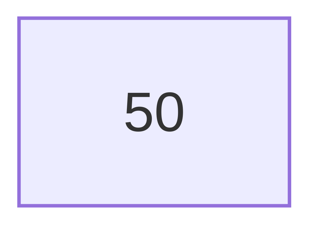
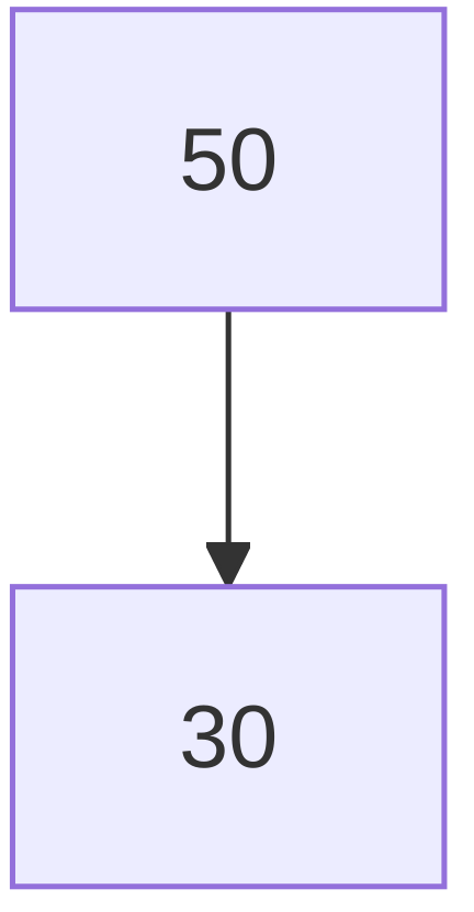
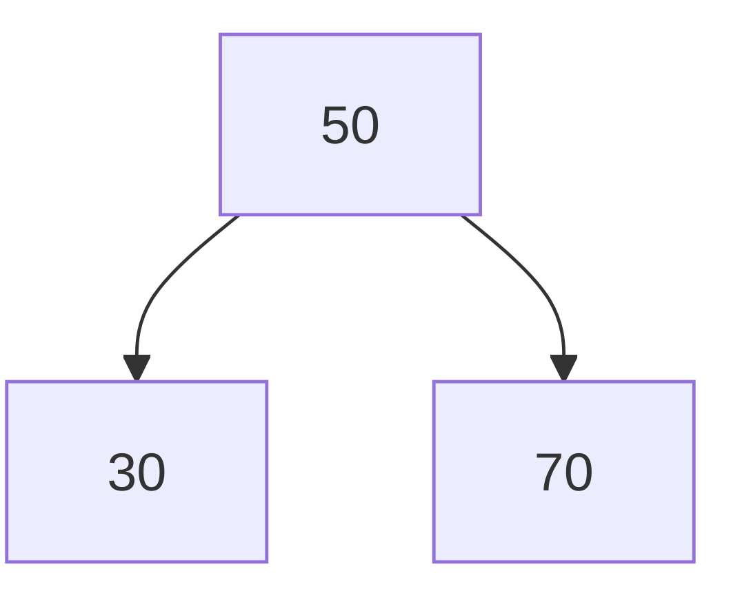
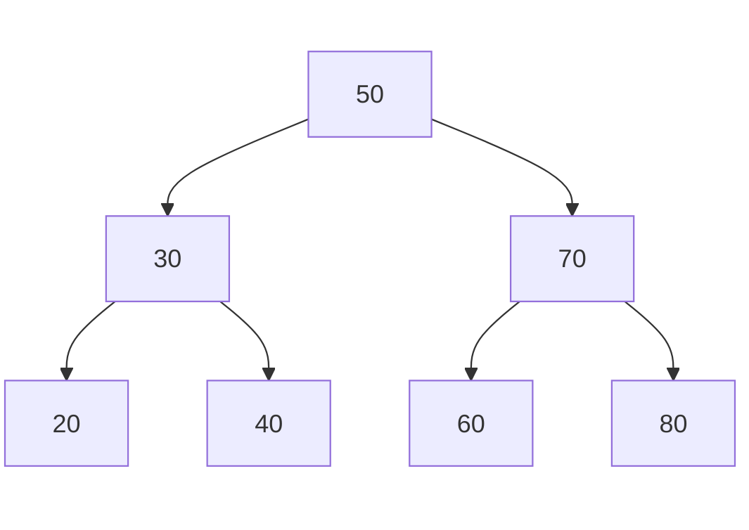
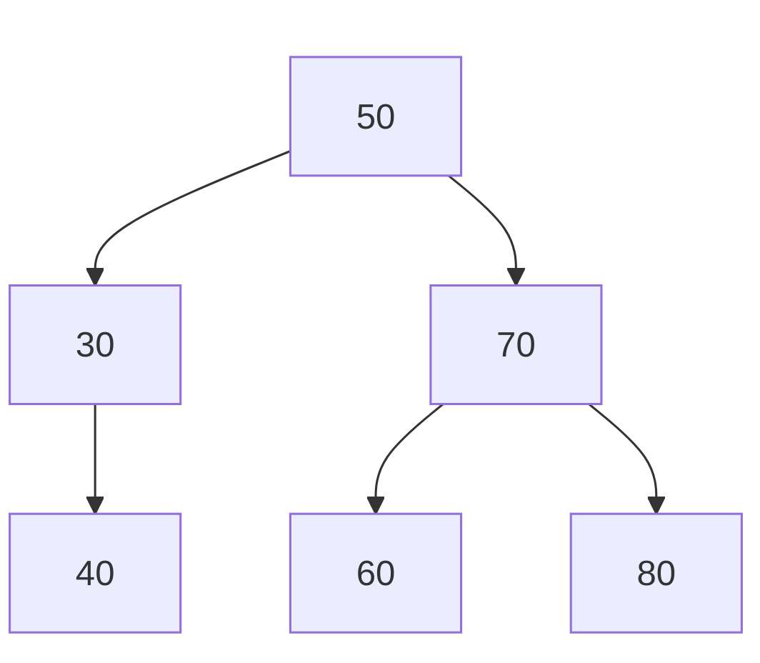
- Insert the following sequence of numbers into an empty BST: 50, 30, 70, 20, 40, 60, 80.
- Represent the tree at each step.
Initial Tree:
After inserting 30:
After inserting 70:
Final Tree After All Inserts:

3. Deletion in BST (40 minutes)
- Deletion Cases:
- Case 1: Node has no children:
- Simply remove the node.
- Case 2: Node has one child:
- Replace the node with its child.
- Case 3: Node has two children:
- Replace the node with its in-order successor (smallest value in the right subtree).
- Case 1: Node has no children:
- Code Example (C++):
cppCopy codeNode* findMin(Node* root) {
    while (root->left != nullptr) {
        root = root->left;
    }
    return root;
}

Node* deleteNode(Node* root, int value) {
    if (root == nullptr) return root;

    if (value < root->value) {
        root->left = deleteNode(root->left, value);
    } else if (value > root->value) {
        root->right = deleteNode(root->right, value);
    } else {
        // Case 1 and 2: Node with one or no child
        if (root->left == nullptr) {
            Node* temp = root->right;
            delete root;
            return temp;
        } else if (root->right == nullptr) {
            Node* temp = root->left;
            delete root;
            return temp;
        }

        // Case 3: Node with two children
        Node* temp = findMin(root->right); // In-order successor
        root->value = temp->value;
        root->right = deleteNode(root->right, temp->value);
    }

    return root;
}
- Graph Visualization:
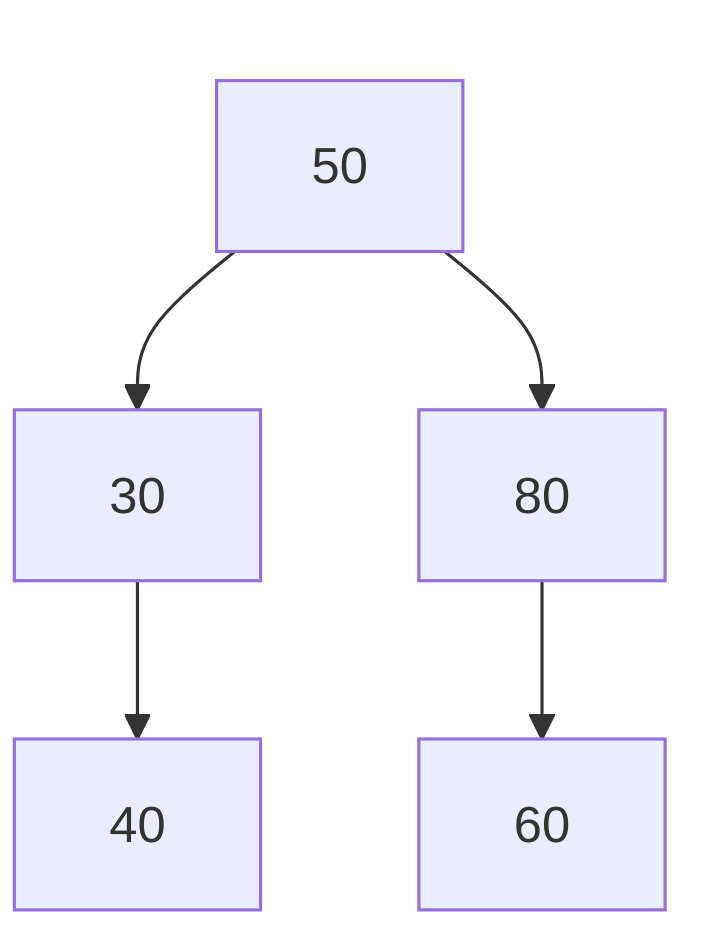
- Start with the final tree from the insertion example.
- Delete the following nodes and show the tree at each step:
- Delete 20 (leaf node).
- Delete 70 (node with two children).
Initial Tree:
After deleting 20:
After deleting 70:
4. Hands-On Exercise (20 minutes)
- Write code to:
- Insert 50, 20, 70, 10, 30, 60, 80.
- Delete 30 and 50.
- Print the tree (pre-order, in-order, and post-order traversals).
- Visualize the resulting tree.
5. Summary and Discussion (10 minutes)
- Recap:
- Properties of a BST.
- Insertion and deletion operations.
- Common pitfalls (e.g., maintaining tree structure during deletion).
- Discussion:
- When is a BST inefficient? (Answer: When it becomes unbalanced.)
- How does this relate to self-balancing trees (e.g., AVL or Red-Black Trees)?
This activity combines theory, visualization, and coding to ensure students grasp how to manage nodes in a Binary Search Tree. The use of Mermaid graphs makes tree transformations intuitive and engaging.